U.S. Census Data Analysis

Project Overview

This project involved a comprehensive analysis of U.S. Census data from 2010 to 2015, focusing on population estimates and geographic classifications across states and counties. The goal was to extract key insights by answering specific analytical questions and visualizing the findings to gain a clearer understanding of demographic and geographic patterns.

Problem Statement

The analysis aimed to answer the following key questions from the U.S. Census dataset:

1. Which state has the most counties in it? (hint: consider the sumlevel key carefully! You'll need this for future questions too.)
2. Only looking at the three most populous counties for each state, what are the three most populous states (in order of highest population to lowest population)? Use CENSUS2010POP
3. Which city has the most counties in it?
4. Which region has the most division in it?

Dataset

The analysis utilized the "census.csv" dataset, which contains population data for counties and states across the U.S. from 2010 to 2015. Key variables used included:

• SUMLEV: Geographic summary level (40 for states, 50 for counties).
• STNAME: State name.
• CTYNAME: County name.
• CENSUS2010POP: Population count from the 2010 Census.
• REGION: Census Region code.
• DIVISION: Census Division code.

The dataset allowed for granular analysis at both state and county levels, providing a rich source of information for demographic insights.

Methodology & Approach

The analysis followed a structured approach using Python and its data science libraries:

1. Data Loading & Initial Inspection: Loaded the `census.csv` dataset into a Pandas DataFrame and performed initial inspections to understand its structure, columns, and data types.
2. Data Filtering: Applied filters based on `SUMLEV` to differentiate between state-level (SUMLEV=40) and county-level (SUMLEV=50) data for targeted analysis.
3. Aggregations & Calculations: Utilized `groupby()` and aggregation functions (e.g., `nunique()`, `sum()`, `nlargest()`) to answer specific questions about county counts, population sums, and geographic divisions.
4. Data Visualization: Employed Matplotlib and Seaborn to create various bar charts that visually represent the key findings, making complex data easily digestible.
5. Interpretation of Ambiguous Questions: Carefully interpreted questions, like "Which city has the most counties in it?", considering the dataset's `CTYNAME` field represents counties, and explained the chosen interpretation.

Key Findings

The analysis yielded several key insights corresponding to the problem statement:

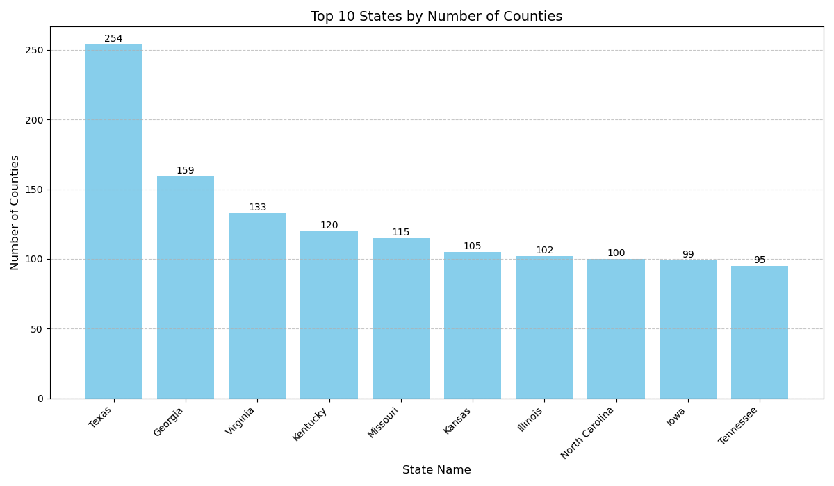
• 1. Which state has the most counties in it?
  • Answer: **Texas** has the highest number of counties, with **254** counties. This highlights its significant number of administrative divisions.
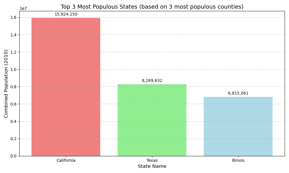
• 2. Only looking at the three most populous counties for each state, what are the three most populous states (in order of highest population to lowest population)?
  • Answer:
    • California: 15,924,150
    • Texas: 8,269,632
    • Illinois: 6,815,061
    This indicates that these states have extremely large population concentrations in their major urban counties.
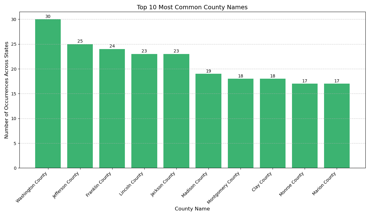
• 3. Which city has the most counties in it?
  • Interpretation & Answer: Given the dataset's structure where `CTYNAME` refers to county names, this question was interpreted as identifying the county name string that appears most frequently across all U.S. states. The most common county name is Washington County, occurring **30** times.
• 4. Which region has the most divisions in it?
  • Answer: The **South** region has the most divisions, with **3** distinct Census divisions. Other regions (Northeast, Midwest, West) each have 2 divisions.

Conclusion

This project successfully demonstrated the ability to extract, analyze, and visualize insights from a structured dataset like the U.S. Census data. By carefully segmenting the data and applying appropriate analytical methods, we were able to answer specific demographic and geographic questions, providing a clearer understanding of the U.S. population landscape.